There is a good reason we are all fascinated with the walkers experiment. For any student of Quantum Mechanics (QM), the interpretation of the QM formalism is at first a puzzling proposal. There is a large suspension of disbelief that needs to take place. Simply put it is ‘counter intuitive’ and most people “shut up and calculate” essentially bowing to the myth that “QM is just very weird”.

How can things be in ‘several states’ at the same time. QM matter must be of a different, slightly magical, nature. It is perhaps best exemplified by paradox of the Schrodinger cat that is both dead and alive, supposedly at the same.

In this post we will apply the formalism of walkers, an emergent model of QM dynamics that comes about from the association of a particle and a wave and show how it sheds a new light on the fundamental interpretation of QM and show that in this interpretation, the cat is simply always dead.

We will also use this formalism to shed light on the typically QM notion of coherence and decoherence.

A brief overview of Walkers.

Walkers are the association of a particle bouncing on a liquid silicon surface and the waves this bouncing creates. Everytime the particle bounces on the surface it creates a standing wave (modeled by a Bessel function in 2D) which in turn drives the particle. The sum of the history of bouncing informs the future bouncing. When the particle bounces it picks up an acceleration due to the gradient of the local surface (like a surfer on a wave). This dynamical system, the association of the particle and its wave exhibits interesting self-quantized dynamics.

A strict interpretation of the deBroglie wave/particle duality.

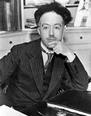
Louis deBroglie, one of the fathers of QM, postulated wave/particle duality. Observing that sometimes matter behaves as a wave and sometimes as a particle, he postulated a relation between the energy of a particle and it’s ‘deBroglie’ wavelength in his PhD thesis. This earned him the Nobel prize in 1929. The walker are a strict implementation of this idea as we have both a particle and its adjoined wave.

Surfers vs Walkers

This point is a little technical but is worth mentioning. The walkers ‘bounce’. Each bounce creates a wave. This is a ‘discrete’ phenomena as opposed to ‘continuous’. We sum a finite number of waves. A continuous phenomena, requiring integration, would be a ‘surfer’. It is worth mentioning because some of the current formalism for the walkers (most notably the Bush formalism we use in this research) is really a ‘surfer’ formalism, assuming a continuous wave creation along the path.The surfer creates the waves it surfs on.

Self-excitation, Self quantization. QM behavior

The dynamics of this system is interesting in it’s path. The particle will self-excite and start ‘walking’ as seen in the video. More importantly to the QM study, some of the behavior observed mimics QM. For example if the particle is submitted to an elastic potential (by way of an EM field) it starts orbiting and showing ‘quantized’ (discrete sets) of possible orbits. The path cannot be “anything” it is quantized by it’s own history, the path creates the path. The history quantizes (by offering a discrete set of possibilities) the future.

Chaotic Dynamics

To understand the solution, pay close attention to the videos from Heligone and the intermittences that appear. The runs captured in matlab by Heligone tell a very clear story. The point is that the orbit goes from trefoils to ovals and sometimes circles. These are the quantized orbits. The change between these orbits is called ‘intermittence’ and is a characteristic signature of chaotic dynamics. The dynamics will randomly change between these stable, discrete, orbits.

Superposition revisited as intermittence

If one observes these objects over long periods of time, one can compute the ‘time’ the particle spends in each orbit. With this mental picture we can revisit QM. It is a different interpretation than QM. In QM, the particle is in ‘several states’ AT ONCE, meaning it would be in the oval and the trefoil at the same time. This is difficult to picture for macro objects such as the cat. In this model, the particle oscillates between those states over time, but NOT AT THE SAME TIME. There is no superposition, just intermittence, an oscillation between the states with certain transition probabilities.

Weights as probabilities.

If one computes the times, one can arrive at the probability one would observe the particle in a particular state. These are transition probabilities. This formalism demystifies the Hilbert space formalism that says that the particle is in all the states with various probabilities. Here there is a logical and simple interpretation for those ‘weights’ they are the probabilities to find the particle in the particular quantized states available to the dynamics. It is simply the time it spends in each quantized orbit.

Schrodinger’s cat is always dead

Let’s revisit the Schrodinger cat paradox in this picture. The idea that a cat would be dead and alive has confused generations of students for the past 100 years and while it makes for good magical mythology it is just false logic in this picture. More importantly, it is the act of observing it that kills the cat. There are several problems with the paradox: a/ we are not in 2 states at the same time. In this model we either are in orbit A or B but not in both at the same time. We oscillate between those states at different times. We are only in ONE state at a time (even if changing rapidly). b/ the category dead/alive are different than intermitting between orbit a and b. Simply put we cannot ‘intermit’ between dead and alive like we can jump back and forth from orbit A to B and vice versa. But ounce you reach “dead”, you stay dead. So essentially the particle would eventually orbit to ‘dead’ state for the cat, and once it has done it, the cat IS DEAD. End of story.

Observation

In this picture the idea that observation is what killed the cat, which is the usual interpretation, is laughable. You didn’t magically kill the cat with your thoughts, the cat died because the particle decayed. End of story.

But Quid of Decoherence and the measurement problem.

This is technical but is the heart of the issue at hand. In QM, the act of observation is what creates the ‘wave collapse’ and ‘decoherence’. The system is classical, not QM after the act of observation.

There is a big difference in the walker system: Essentially in the case of walkers, the observation of the particle (here in silicon and silico) DOES NOT DESTROY THE FIELD. This is the important part. If the act of measuring interferes with the field (uses tools that are on the order of magnitude of the deBroglie wavelength), which is the case for ‘classical QM” (remember the observation of slits in the Young double slit experiments is enough to destroy the QM result) then one loses the chaotic dynamics induced by the field. Observing a QM dynamic induced by a ‘field’ destroys the field. So the QM dynamics stop the moment we ‘observe’ them. The measurement problem is at the heart of our problems with QM.

The notion of ‘coherence’ and ‘decoherence’ which is usually magically associated with the existence of ‘superposition’ and it’s disappearance (the mythical wave collapse) is very simply the existence of intermittence due to chaotic dynamics. “Coherence” in the walker/surfer picture is the existence of the association of the particle and the field and the resulting chaotic/intermittent dynamics. Destroying the field destroys that dynamic. the dynamic becomes classical dynamics and ceases to be quantum dynamics. Observing a QM system destroys its QM dynamics if one destroys the field. Decoherence is the destruction of the wavefield self-generated by the particle bouncing about and thus the end of the QM dynamic. QM dynamics is a chaotic dynamics brought about by memory of its past via a wavefield that is easy to destroy.

And that is all there is to it.

A brief historical philosophy consideration

In conclusion, the latest Couder work, simply explains many of the QM behaviors and the magical coherence/decoherence and seems very simple in retrospect. Why wasn’t this ‘particle/wave’ duality taken to it’s logical conclusion by the founding fathers of QM? One has to project back to the Solvay conference in 1927, where deBroglie proposed these ideas and was shot down by the Copenhagen school. It is not hard to see why.

To make headway with these models (which we do in the 21st century) one needs the formalism of chaotic dynamics (which was developed in the 80’s and 90’s) and powerful computers to run the integration as there is little headway to be had analytically. In short, while philosophically satisfying, the wave/particle duality interpretation is difficult from a practical standpoint. In front of this model there was the straightforward (if magical) interpretation of the Copenhagen school: namely a vectorial superposition of states in a abstract ‘hilbert space’ that could give practical results in calculation. The ‘shut up and calculate’ mentality was justified as it gave us the atom bomb, most the technological advances of the late 20th century (think lasers, computer spin storage etc) and the CERN Higgs. The practical nature of the formalism was justification enough. The interpretation was secondary.

There is no magic.